Efficient and accurate filtering of polygonal shapes can be achieved with closed-form solutions based on Green's theorem with piecewise-polynomial filters (e.g. box/bilinear/bicubic).
Instead of relying on pixel-approximations or super-sampling to achieve filtering effects, it is possible to directly compute the exact filtered coverage, by:
- Breaking the polygon up into smaller (usually-pixel-sized) clipped polygons
- Evaluating the filter integral directly for each clipped polygon
Furthermore, this can be done on the GPU, and is demonstrated in WebGPU in this article (if it is enabled).
Introduction
Rasterization is the process of converting vector graphics into pixel data. When rendering a polygon, the rasterizer needs to determine how much the polygon covers each pixel, so that it can determine the polygon's contribution to the pixel.
A fast approach, given many polygons, is to see how much of each polygon is contained within the box of each pixel. However, when polygons overlap, this approach can lead to over-coverage, and can result in incorrect blending known as conflation artifacts. To avoid this, it is ideal to compute exact (non-overlapping) coverage, but it can also be approximated by super-sampling.
Filtering is a key component of anti-aliasing, which is used to reduce the visual artifacts that occur when rendering high-frequency content at a lower resolution.
Browsers' built-in anti-aliasing for SVG and Canvas shapes, particularly when animated, usually does not include a significant amount of filtering. When displaying certain shapes, this results in aliasing artifacts that can be distracting or even misleading.
Filters
While a pixel is not a little square, a simple way to get a coverage value is to use the area of the polygon that covers the pixel. This is equivalent to applying a box filter to the polygon, which is the simplest form of filtering.
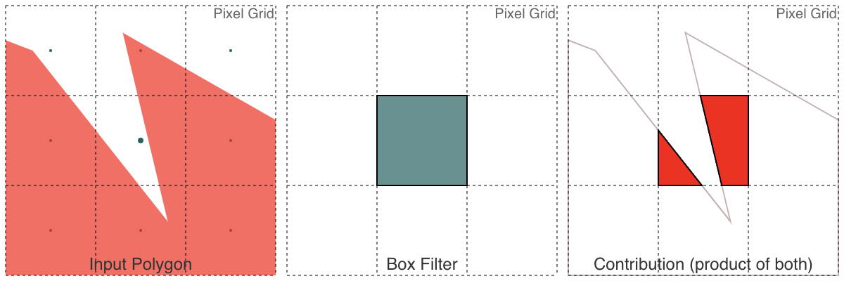
While the box filter results in a sharp result, it can result in spatial aliasing artifacts. These can be reduced by using other filters. Instead of taking the area of the polygon that covers a square around the center of the pixel, others will evaluate a different weighted function over the polygon.
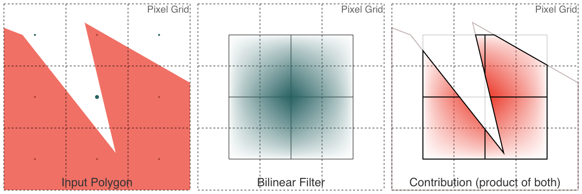
The bilinear and Mitchell-Netravali (bicubic) filters are two common filters that are used in practice, and both are piecewise-polynomial filters.
These piecewise-polynomial filters are equivalent to taking the integral of the piecewise-polynomial function within the polygon, where the filter function is centered at where a sample is being taken. The box filter is equivalent to taking the integral of an indicator function that is 1 within the square, and 0 outside.
In particular, each of the above filters has one or more clipped areas of the polygon that will
Green's Theorem and Polygons
We will dive into the math behind how we can evaluate the integral of a filter over a polygon using Green's Theorem. For more related results, see Alpenglow's integrals for anti-aliasing.
Overall:
- To evaluate an integral (i.e. a filter) over a shape, we can instead evaluate an integral over the boundary.
- For polygons, this means we can evaluate an expression for each edge (given $x_0$, $y_0$, $x_1$, and $y_1$), and sum those up.
- If the integrand is a polynomial, we get a closed-form solution that can be evaluated directly.
Using Green's Theorem, we can convert a double integral over a region into a line integral over the (closed, oriented counter-clockwise) boundary of the region:
$$ \oint_P\left(L\,\frac{dx}{dt}+M\,\frac{dy}{dt}\right)dt=\iint_P \left( \frac{\partial M}{\partial x}-\frac{\partial L}{\partial y} \right)\,dx\,dy $$
for curves parameterized on $t$.
For polygons, this means that if we can evaluate a line integral over each line segment (between $(x_i,y_i)$ and $(x_{i+1},y_{i+1})$, finishing with $(x_i,y_i)$ to $(x_0,y_0)$), we can sum up each edge's contribution to evaluate the double integral for the region inside the polygon. Each line segment is parameterized curve:
$$ x=x(t)=(1-t)x_i+(t)x_{i+1}=x_i+t(x_{i+1}-x_i) $$ $$ y=y(t)=(1-t)y_i+(t)y_{i+1}=y_i+t(y_{i+1}-y_i) $$ for $0 \le t \le 1$, with the derivatives: $$ \frac{dx}{dt}=x_{i+1}-x_i $$ $$ \frac{dy}{dt}=y_{i+1}-y_i $$ Note:
- If we reverse an edge (swap its endpoints), it will swap the sign of the contribution to the integral (a polygon can make a degenerate turn and double-back precisely, with no contribution to area). Thus for terms, swapping $i$ and $i+1$ will swap the sign of the contribution. This means that polygons with holes can be evaluated by visiting the holes with the opposite orientation (clockwise).
- This is evaluated on closed polygons, so any terms that only depend on one endpoint will cancel out (e.g. $x_i^2y_i$ and $-x_{i+1}^2y_{i+1}$ will have their contributions cancel out, since both of those will be evaluated for every point in the polygon). It is useful to adjust the coefficients to these terms, since they can allow us to factor the expressions into simpler forms (e.g. the Shoelace formula below).
We can pick $L$ and $M$ below: $$ L=(n-1)\int f\,dy $$ $$ M=(n)\int f\,dx $$ so that $$ \iint_P \left( \frac{\partial M}{\partial x}-\frac{\partial L}{\partial y} \right)\,dx\,dy= \iint_P \left( (n)f - (n-1)f \right)\,dx\,dy= \iint_P f\,dx\,dy $$ for any antiderivatives and real $n$, since the double integral will then be integrating our function $f$. It turns out, evaluating Green's Theorem over line segments for polynomial terms for any linear blend (any $n$) of $L$ and $M$ will differ only in the "canceled out" terms, so each edge's contribution will be the same.
Integrating Polynomials over Polygons
If we zero out all of the canceled terms, it turns out that we can evaluate the integral of any polynomial term $x^my^n$ over a polygon $P$ by summing up the contributions of each edge:
$$ \iint_Px^my^n\,dx\,dy=\frac{m!n!}{(m+n+2)!}\sum_{i}\left[ (x_iy_{i+1}-x_{i+1}y_i) \sum_{p=0}^m\sum_{q=0}^n \binom{p+q}{q}\binom{m+n-p-q}{n-q}x_i^{m-p}x_{i+1}^py_i^{n-q}y_{i+1}^q \right] \tag{1} $$
This was first discovered by Soerjadi in 1968. The contributions of each term can be summed up individually to integrate arbitrary polynomials.
e.g. for $x^4y^2$ in matrix form:
$$ \iint_Px^4y^2\,dx\,dy= \frac{1}{840} \sum_{i} \left( (x_iy_{i+1}-x_{i+1}y_i) \begin{bmatrix} x_i^4 & x_i^3x_{i+1} & x_i^2x_{i+1}^2 & x_ix_{i+1}^3 & x_{i+1}^4 \end{bmatrix} \begin{bmatrix} 15 & 5 & 1\\ 10 & 8 & 3\\ 6 & 9 & 6\\ 3 & 8 & 10\\ 1 & 5 & 15 \end{bmatrix} \begin{bmatrix} y_i^2\\ y_iy_{i+1}\\ y_{i+1}^2 \end{bmatrix} \right) $$
Any polynomial-based (windowed or not) filter can be evaluated over a polygon with this approach. It may be feasible to approximate Gaussian/Sinc filters with polynomials, or find iterative approaches to converge to the integral.
Integrals for Filters
Box Filter (Area)
As seen above, the box filter is equivalent to a step function that is 1 within the box and 0 outside. When a polygon has been clipped, this is equivalent to evaluating the integral of $1$ inside the polygon (i.e. computing its area).
For $x^0y^0=1$, with adding some canceling terms to better factor, we will obtain the Shoelace formula for finding the area of a polygon: $$ area_P=\iint_P1\,dx\,dy= \frac{1}{2} \sum_{i} (x_i+x_{i+1})(y_{i+1}-y_i) $$
This formula will be evaluated (with the appropriate order and orientation) for every edge ($x_i$, $y_i$, $x_{i+1}$, $y_{i+1}$) along a polygon. The sum will be the area of the polygon.
Bilinear Filter
The bilinear filter is equivalent to integrating the tent function over the polygon. As seen above, this is broken into 4 quadrants, each of which is a polynomial function.
Without loss of generality, we can focus on computing the integral solely in the $0\le x\le1,0\le y\le1$ quadrant. The integrand is thus:
$$ (1-x)(1-y)=xy-x-y+1 $$
This is a weighted sum of the terms $x^1y^1$, $x^1y^0$, $x^0y^1$, and $x^0y^0$. We can sum up the weighted contribution of the corresponding terms from $\tag{1}$, resulting in the following evaluated line integral:
$$ \frac{1}{24}\sum_{i}(x_iy_{i+1}-x_{i+1}y_i)(12-4( x_i+y_i+x_{i+1}+y_{i+1})+2(x_iy_i+x_{i+1}y_{i+1})+ x_iy_{i+1}+x_{i+1}y_i) $$
This formula will be evaluated (with the appropriate order and orientation) for every edge ($x_i$, $y_i$, $x_{i+1}$, $y_{i+1}$) along a polygon (clipped to the unit square). The sum will be the integral of this quadrant of bilinear filter over the polygon (with the filter centered at the origin). Coordinate transformations can be used to evaluate the other quadrants (applying the absolute value to inputs).
Note that the polygon needs to be clipped so that it is fully contained within the unit square.
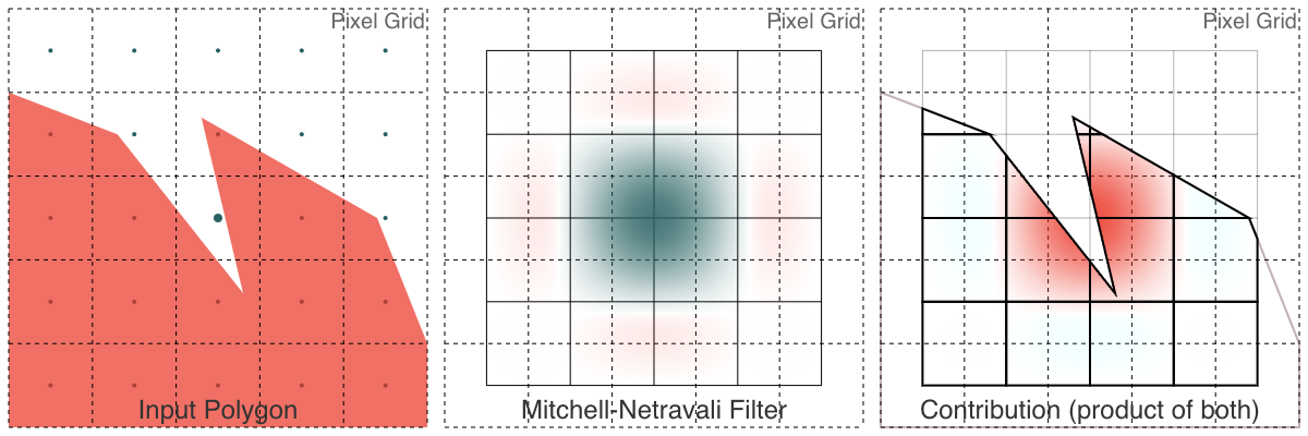
Mitchell-Netravali Filter
The Mitchell-Netravali filter family, commonly referred to as "bicubic", is a piecewise-polynomial filter that that has a larger support, and includes negative lobes to reduce artifacts. It has 16 different polynomial pieces, which will require the integral evaluation of 3 different pieces.
We choose to use the "Mitchell-Netravali" filter (specifically with constants $B=1/3$ and $C=1/3$). It is separable and symmetric, so the integral is equal to $f(x)f(y)$, combining 1-dimensional kernels. The two polynomial chunks we get (assuming a $t > 0$) are:
$$ f_0(t)=\frac{1}{6}\left(7y^3-12t^2+\frac{16}{3}\right) $$
for $0\le t\le1$, and:
$$ f_1(t)=\frac{1}{6}\left(-\frac{7}{3}y^3+12t^2-20t+\frac{32}{3}\right) $$
for $1\le t\le2$.
Taking into account symmetry, this gives us three different polynomial chunks we will need to evaluate:
- $f_0(x)f_0(y)$
- $f_0(x)f_1(y)$
- $f_1(x)f_1(y)$
Since the others can be obtained by reversing signs and/or reflection with swapping x/y input.
All three of these can be evaluated using the formula $\tag{1}$, since they are simply polynomials in $x$ and $y$. Notably:
$$ f_0(x)f_0(y)= \begin{bmatrix}1 & x & x^2 & x^3\end{bmatrix} \begin{bmatrix} \frac{64}{81} & 0 & -\frac{16}{9} & \frac{28}{27}\\ 0 & 0 & 0 & 0\\ -\frac{16}{9} & 0 & 4 & -\frac{7}{3}\\ \frac{28}{27} & 0 & -\frac{7}{3} & \frac{49}{36} \end{bmatrix} \begin{bmatrix}1\\y\\y^2\\y^3\end{bmatrix} $$
$$ f_0(x)f_1(y)= \begin{bmatrix}1 & x & x^2 & x^3\end{bmatrix} \begin{bmatrix} \frac{128}{81} & -\frac{80}{27} & \frac{16}{9} & -\frac{28}{81}\\ 0 & 0 & 0 & 0\\ -\frac{32}{9} & \frac{20}{3} & -4 & \frac{7}{9}\\ \frac{56}{27} & -\frac{35}{9} & \frac{7}{3} & -\frac{49}{108} \end{bmatrix} \begin{bmatrix}1\\y\\y^2\\y^3\end{bmatrix} $$
$$ f_1(x)f_1(y)= \begin{bmatrix}1 & x & x^2 & x^3\end{bmatrix} \begin{bmatrix} \frac{256}{81} & -\frac{160}{27} & \frac{32}{9} & -\frac{56}{81}\\ -\frac{160}{27} & \frac{100}{9} & -\frac{20}{3} & \frac{35}{27}\\ \frac{32}{9} & -\frac{20}{3} & 4 & -\frac{7}{9}\\ -\frac{56}{81} & \frac{35}{27} & -\frac{7}{9} & \frac{49}{324}\\ \end{bmatrix} \begin{bmatrix}1\\y\\y^2\\y^3\end{bmatrix} $$
Long story short, evaluating $\tag{1}$ for these, we get some reasonably long expressions that can be evaluated directly.
For example: $f_0(x)f_0(y)$ results in:
1/51840 ($x_0$ - $x_1$) (3 $y_0^4$ (896 + 735 $x_0^3$ + 45 $x_0^2$ (-32 + 7 $x_1$) + 15 $x_0$ $x_1$ (-32 + 7 $x_1$) + 3 $x_1^2$ (-32 + 7 $x_1$)) + 128 (160 + 3 $x_0^2$ (-20 + 7 $x_0$) + 6 $x_0$ (-20 + 7 $x_0$) $x_1$ + 9 (-20 + 7 $x_0$) $x_1^2$ + 84 $x_1^3$) $y_1$ - 96 (80 + 3 (-4 + $x_0$) $x_0^2$ + 12 (-4 + $x_0$) $x_0$ $x_1$ + 30 (-4 + $x_0$) $x_1^2$ + 60 $x_1^3$) $y_1^3$ + 3 (896 + 3 $x_0^2$ (-32 + 7 $x_0$) + 15 $x_0$ (-32 + 7 $x_0$) $x_1$ + 45 (-32 + 7 $x_0$) $x_1^2$ + 735 $x_1^3$) $y_1^4$ + 6 $y_0^2$ $y_1$ (-16 (80 + 30 $x_0^3$ + 36 $x_0^2$ (-2 + $x_1$) + 12 (-3 + $x_1$) $x_1^2$ + 9 $x_0$ $x_1$ (-8 + 3 $x_1$)) + (448 + 3 (35 $x_0^3$ + 9 $x_0$ $x_1$ (-16 + 7 $x_1$) + $x_1^2$ (-96 + 35 $x_1$) + $x_0^2$ (-96 + 63 $x_1$))) $y_1$) + 4 $y_0$ (32 (160 + 84 $x_0^3$ + 9 $x_0^2$ (-20 + 7 $x_1$) + 6 $x_0$ $x_1$ (-20 + 7 $x_1$) + 3 $x_1^2$ (-20 + 7 $x_1$)) - 24 (80 + 12 (-3 + $x_0$) $x_0^2$ + 9 $x_0$ (-8 + 3 $x_0$) $x_1$ + 36 (-2 + $x_0$) $x_1^2$ + 30 $x_1^3$) $y_1^2$ + 3 (224 + 21 $x_0^3$ + 15 $x_1^2$ (-16 + 7 $x_1$) + 9 $x_0^2$ (-8 + 7 $x_1$) + 3 $x_0$ $x_1$ (-64 + 35 $x_1$)) $y_1^3$) + 12 $y_0^3$ (32 (-20 + 7 $y_1$) + 3 (5 $x_0^3$ (-32 + 7 $y_1$) + $x_1^2$ (32 - 8 $x_1$ - 24 $y_1$ + 7 $x_1$ $y_1$) + 5 $x_0^2$ (64 - 16 $x_1$ - 16 $y_1$ + 7 $x_1$ $y_1$) + $x_0$ $x_1$ (128 - 32 $x_1$ - 64 $y_1$ + 21 $x_1$ $y_1$))))
Common terms can be factored out, speeding this up somewhat, but it is still less efficient than the bilinear case.
Blurring
While the typical filter size is small (and may slightly blur the edges of a polygon), it is possible to dramatically expand the size of the filter (computed for each pixel) to intentionally blur the polygon. Generally when this is done, each of the clipped piecewise-polynomial sections will NOT overlap with those of other pixels, so it takes a bit more computation and clipping to evaluate the integral.
Note that large blur radii are not too much more expensive than small ones, it depends on the geometry of the scene. Each pixel will need to have access to the geometry and shading within its support region. The demo above is slowed down by the GC-hungry CPU procedure that computes occlusion.
Implementation
Alpenglow has both a CPU and WebGPU implementation of this filtering during rasterization. Both approaches will typically hierarchically clip the polygon into smaller pieces (on the GPU, using the edge-clipped form noted in Alpenglow documentation).
On the GPU, this has been done so far by clipping things into approximately 256x256 tiles, and then further into approximately 16x16 sub-tiles, at which the final clipping can be done during the rasterization. There are multiple approaches (using WebGPU compute shaders) to doing this efficiently, it is something I'm working on!
The clipped regions need to be expanded by the radius of the filter's support. For example, the bilinear filter will need to be expanded by 1 pixel in each direction, and the bicubic filter will need to be expanded by 2 pixels (from the pixel centers).
It turns out that for normal filter sizes, the clipped regions for different pixels will overlap (e.g. for bilinear, pixel 0,0 and 1,1, one of the quadrants will be shared). Thus on the GPU, a workgroup can compute a 16x16 grid of clipped polygons, evaluate all of the 4 potential integrals, and for speed can evaluate the color of that region. Then those integrals can be used to blend the results into a 15x15 section of pixels.
This method is the most effective when the occlusion problem has already been solved (e.g. with a computation-area geometry approach like Alpenglow). With that type of approach, the clipped regions will not overlap, and the integrals can be evaluated directly.